Doge & Altcoin in Excel (Simple!)

An easy way to fetch up-to-date market data about Doge coin and (almost) any other crypto coin in Excel.

There are many methods to get web data and specifically crypto market data into Excel. I find this one to be simple, reliable, and free.

Pros for this method:

• Data is from the great source of CoinMarketCap.com
• This method is easy to use for non-developers
• This method works on MacOS and Windows

Cons for this method:

• Does not work on mobile and web
• Requires access to a local .iqy file stored on your machine
• Requires dedicated helper-tab for each coin you need to fetch

---

The Basics:

To fetch the data we will use Microsoft’s “Web Query”, this requires writing a file with .iqy file extension on your local machine.

It would seem that Microsoft is not pushing this feature and maybe even considering deprecating it for one of the alternatives, but for now this works perfectly.

Documentation is a bit limited by you can read about it from non official sources, such as –

• Excellent post by Justin James from 2006.

---

Getting Start – Write an iqy file:

Using your preferred text editor, write down the following content to a local file, and call it “Crypto Assets.iqy”.

• The file name and location are not important as long as you remember them

The content for “Crypto Assets.iqy”:

WEB
1
https://coinmarketcap.com/currencies/["Crypto Asset"]/

Selection=AllTables
Formatting=None
PreFormattedTextToColumns=True
ConsecutiveDelimitersAsOne=True
SingleBlockTextImport=False
DisableDateRecognition=False
DisableRedirections=False

Setup web query in Excel:

• Open you Excel worksheet, add new Sheet, and call it “DogeCoin”.
• Navigate in the top menu options to find –

Data → Get External Data → Run Web Query…

Select “Run Web Query…”

• A prompt will open to ask you for for location of the iqy file. Find you “Crypto Assets.iqy” file and open it.
• A second prompt will ask you for location to dump the output. Accept the defaults.
• A third prompt will ask you for the name of the asset you need.
  • In this example, we want the current price of DogeCoin so please type “dogecoin”
  • Make sure to type it correctly
  • Also, make sure to check the check-box for “Use this value/reference for future refreshes”
  • Finally, click “Ok”

Select “Crypto Asset”

• Excel will fetch the data. If all is well you should see the following:

DogeCoin price today

• Every time you need updated number just hit navigate to the Data menu and hit Refresh All.

Refresh All Data

• The same can be done for other crypto assets covered by CoinMarketCap. Just make sure to spell the asset name in full and correctly. Try out “bitcoin”, “ethereum”, “shiba-inu”, or any other asset.
• This basic concept can be automated, and enhanced in VBA, but that is beyond the scope of this post.

Thanks for reading and I hope this is useful.

Crypto data in Excel

Historically, I’ve used a not-so-simple Excel VBA code that will fetch Cryptocurrency data from the good people at coinmarketcap.com. This is probably still the right way to go for many use cases.

In addition, Excel now has a built-in support for fetching crypto currency data, with a very simple / no-coding-required option.

In this blog post we will first look at how to use this option and then review a set of Q&A demonstrating the limits of this option and wondering about how this could become a lot better.

Step 1: Type your From/To ticker

The first thing we need to do is select the ticker.

It is a cell in your Excel with a string representing a pair of a Crypto coin on the left and a Fiat coin on the right for one of the supported combinations of From/To.

For example, to get the US dollar value of Bitcoin, you would write something like BTC/USD. The data source also support other conversions such as Bitcoin to Euro , BTC/EUR and others.

Step 2: Mark this Cell as a Stock Ticker

The second step is to tell Excel that this is a Stock field.

For that go to the data tab, and select the stocks option. The cell will change and include a new Stock logo on its left.

Step 3: Select the data fields

Now you will notice to the right of the cell an option to select columns.

Available columns for Crypto coins are different from regular Stocks.

The following fields are available as of today (May-2021):

• 52 week high
• 52 week low
• Change
• Change (%)
• Currency
• From currency
• High
• Instrument type
• Last trade time
• Low
• Name
• Open
• Previous close
• Price
• Ticker symbol

Once you selected the fields, they will appear on the right side of the ticket and you are done.

Step 4: Refresh the data

The data in these cells will not automatically update.

To refresh the data go back to the data tab and hit the “Refresh All” button.

You can do the same also in VBA code by using the function: ThisWorkbook.RefreshAll

For example, you could write event handler that is activated every time the file is opened and automatically refresh the data, by implementing Workbook_Open().

And that is all to it.

The rest of this doc includes few Q&A I asked myself and wanted to share.

Which Excel versions and plans support this?

Microsoft states in one article that this feature is included in “Excel for Microsoft 365 Excel for Microsoft 365 for Mac Excel for the web”. And in a second article it clarifies that the feature is available only for users with “Microsoft 365 accounts”. Finally, in a closely related third article about STOCKHISTORY it is claimed that it requires “requires a Microsoft 365 Personal, Microsoft 365 Family, Microsoft 365 Business Standard, or Microsoft 365 Business Premium subscription”.

A bit confusing.

I think that it means that you need an active Microsoft Office 365 subscription, and it can be used only with the Excel for Windows, Mac and Web. Not the mobile versions.

Can we trust the accuracy of their information?

That is a good question. I personally will not be comfortable to use this information for real-time trading. The documentation for the stocks data source just state “information is provided by another company” and refer to Refinitiv as that vendor.

However, they do not list exactly the way the data is aggregated, for example, what is the lag time for the current price, is the the current price based on aggregated latest transaction from multiple trading exchanges, which exchanges are included etc. As a result the accuracy of the data is unclear and should be used for applications, such as trading, that require an almost real-time data.

What Crypto Tickers are supported?

The information about that is also limited. From trial and error we can say that the following tickers are supported:

• Bitcoin (BTC)
• Ethereum (ETH)
• XRP (XRP)

Every other ticker I tried did not work. Including the following popular tickers:

• Binance Coin (BNB)
• Dogecoin (DOGE)
• Cardano (ADA)

Can I get historical information about supported tickers?

Yes, the same tickers are supported with the function STOCKHISTORY and it is very easy to use. I will dedicate a future entry for that use case.

Summary

All in all, using the crypto data is currently fairly limited in terms of the coverage. Quality of data may also be insufficient for real-time trading purposes. However, if you are looking for various data analysis options for Bitcon, Etherium, or XRP, this is a very easy to use and useful tool.

Read more at the Microsoft site with “Get A Stock Quote“, the exact same expereince is available for Cryptocurrencies.

UPDATE: May 22nd, 2021.

Good comment that there are (very) few additional supported tickers. The full list includes just 5 coins and there are –

• Bitcoin (BTC)
• Ethereum (ETH)
• XRP (XRP)
• Bitcoin Cash (BCH) – Updated
• Litecoin (LTC) – Updated

UPDATE 2: May 31st, 2021.

I received a great question about the comment at the top on how to easily get Crypto data into Excel for any asset, or at least any asset that is covered by CoinMarketCap.

Here is a second entry dedicated for that Doge & other Altcoins in Excel.

iPhone swipe to Delete emails

Here is annoying little problem that I’m sure you have seen:

By default, in iPhone / iOS the swipe gesture in the mail app is Archive and not Delete.

iOS Mail archive on swipe

The actual delete operation is hidden under the More button and you have to half swipe the email entry, click on More, and only at that sub-menu you can find the Delete button.

No doubt annoying!

Luckily there is a hidden option to change it.

Let’s see how-to set up the iPhone mail app to offer “swipe to delete” option:

1. Open the Settings app and find the Mail item.
2. Scroll down and find the Accounts item and select the account you would like to change.
3. Click on the > near the account name.
   
4. Select the Advanced option.
   
5. Find the options for Move Discarded Messages Into and change the value there to Delete Mailbox.
   
6. Make sure to click on the back and finally click on the Done option.
   

If you followed these 6 steps (way too ridiculous) and specifically clicked on the Done, your mail should start to behave nicely and offer you an easy way to swipe emails to delete and not the default archive.

iOS Mail delete on swipe

Enjoy!

NodeJs and Apache Cassandra

The next topic for my project was learning about alternative ways for interaction between NodeJs and the Apache Cassandra database.

As a background I am new to the Apache Cassandra environment. In fact, my recent background is in MEAN (MongoDB, ExpressJs, AngularJs, NodeJs). In that world the mapping between MongoDB documents and NodeJs artifacts is well understood and frankly it is one of simplest and most natural Object-Database Mapping (ODM) that I have seen. I am a fan of that approach.

It is not perfect and there is always a tradeoff of productivity vs. efficiency. In previous projects we have found a middle ground where most of the work was done with Mongoose letting the package do its magic and letting us focus more on our application, and only if and when needed, overwriting these commands, getting into the dirty details and implementing optimizations to the needed degree. As the saying goes “keep simple things simple and make complex things possible”.

With that in mind let’s look at the top packages I am using for my NodeJs-Cassandra project:

The first excellent package to consider is DataStax Node.js Driver for Apache Cassandra. Everyone simply call this the cassandra-driver and you can find it here. I found the package to be stable, complete and regularly updated. It provides a direct access to the Cassandra Query Language also known as CQL.

As a very simple example, here is a call to fetch all employees in a department:

The two aspects to highlight is the connection to the database:

var db = new cassandra.Client(
{ contactPoints: ['127.0.0.1'],
protocolOptions: {port: 9042},
keyspace: 'myDB'});

And the call to execute a command (in this case “SELECT” command):

var query = 'SELECT * FROM employees WHERE department = ?';
db.execute(query, [department], function(err, result)...

Note that when executing a command there is a method here to pass parameters to the command. The parameters use are marked with question-mark character inside the CQL command. The values are passed to the execute command as an array of ordered values (i.e. the order in which the the question-marks appear in the command).

All of this is simple enough and useful but it requires me to get into the CQL level and implement manually a set of classes to map database entities to NodJs artifacts. I intend to use this package directly every time there is a need to get to the deeper command level optimization. This is for the complex cases.

Back to the MEAN background, what about the simple cases? Is there a way to have a basic object mapping done transparently, something similar to Mongoose for MongoDB in the MEAN world?

Not to worry. Someone already built a package for that. It is called Cassie-ODM or simply Cassie and it currently in Beta. I gave it a run and liked it a lot. More on that next time.

Tesla really delivering the Model X!

A small confession: Tesla is my unfulfilled dream car. The car I wish to have when I grow-up and can afford myself. Or when the car itself becomes affordable (Model 3?). As such, I monitor the developments and rumors around Tesla all the time.

At the end of 2015 it was the first time I read that Tesla started to ship the Model-X to customer but they are doing that very slowly and experiencing some mechanical issues that they try to solve on-the-fly. For me it was more of a rumor as I am from the east coast and I have yet to see in my own eyes such car in action on the road.

Well today it changed. Today, walking down the streets of Boston I saw for the first time a Tesla Model-X car driving and then parking just like any other regular car.

And it was with the falcon-wing doors open! Awesome!

 

 

Excel Bi-Directional Temperature Converter

A revised version of this content is now available at blog.officewizkid.com

---

I recently received a question on how to develop a bi-directional temperature converter in Excel. Sounds simple enough but the trick here is the bi-directional statement.

The requirement is as follows:

Let’s assume that Cell B4 represents temperatures in Fahrenheit and Cell D4 represents temperatures in Celsius. Changing one of them will need to automatically change the other one.

The end result should look like the following:

Developing an expression that can do a one-directional conversion form Fahrenheit to Celsius is easy. Just type in D4 the expression:


=(B4-32)*5/9


Developing an expression that can do the reverse (still a one-directional conversion) form Celsius to Fahrenheit is easy. Just type in B4 the expression:


=D4*9/5+32


But doing both is much tougher. It creates bi-directional dependency between two cells that as far as i can tell can not be done with simple expressions.

The workaround I found is by going down-level to the VBA level and writing a macro to handle a “worksheet change” event. The event will be triggered every time a cell is changed, making this solution a little bit heavy when dealing with large Excel files. It also requires the Excel to be saved as .xlsm or Excel Macro-Enabled Workbook.

Here is a capture of the code:

Let’s review these statements one by one.

First please open the VBA editor in Excel (see old post about that) and use the drop-down lists to first select “Worksheet” and then “Change”. This will generate for you an empty Private Sub called Worksheet_Change.

The logic here is not too complex and has two parts:

Check that the B4 (or D4) cell was part of the Target change range, for that we check if the intersection between Target and “B4” is not empty.


If Not Intersect(Target, Range("B4")) Is Nothing Then


Next we use the “ActiveSheet.Range” function to select cell “D4” and set its value based on conversion calculation as a function of “B4” value.


ActiveSheet.Range("D4").Value = (ActiveSheet.Range("B4").Value - 32) * 5 / 9


Once completed, we can exit from that Sub.

 

Document Instpector on Mac?

I read today a blog entry regarding the hidden information in Office document and what can be done about it (Do You Know What’s Hiding in Your Documents?).

From a personal experience, especially in business negotiation and contracts, it is kind of surprising to see what can be extracted out of a seemingly clean Word document that the author did not really planned to exposed.

Microsoft has a built-in tool to clean all of that called “Document Inspector”. The tool look easy to use and similar functionality is available for Word, Excel, and PowerPoint.

But I was not able to find the tool or the menu option on my Mac… A google search reveal that this capability is simply not there. I’ve seen multiple discussions about this, like this one – Using document inspector to find personally identifiable information.

As a user of a Mac I find these missing capabilities as a real annoyance. I just hope that Microsoft will take that to heart and start to complete these items…

Basic Pivot Table Example

Microsoft describes PivotTables as “A PivotTable report is useful to summarize, analyze, explore, and present summary data. A PivotChart report can help you visualize PivotTable report summary data so that you can easily see comparisons, patterns, and trends. Both reports enable you to make informed decisions about critical data in your enterprise. The following sections provide an overview of PivotTable and PivotChart reports.” (see here).

And indeed PivotTable is a query tool that quickly generates reports on top of a base table of data. Once you get the basics, it is easy, interactive and very useful tool to know.

As always, let’s see that ability in a simple example:

Let’s assume we have a detailed report of product sales transactions. The report has a lot of information about each transaction, including the product code, the geo, the channel, and the amount.

And we want to run reports and analyze this date. We do that by creating Pivot Table like this:

Select the entire data area and go to the “Data” menu and select “PivotTable…”. A menu like below will open:

Adjust the range if needed and for this simple example just leave all other parameters without a change.

The result is a new sheet that looks like this:

Now we can dynamically select items to display and to summarize.

The simplest example: Let’s create a report of the total sales by GEO.

1. In the “PivotTable Builder” dialog, Drag & Drop the “Geo” field to the “Row Labels”.

2. Drag & Drop the “Price” field to the “Values”. By default the Count function will be applied.

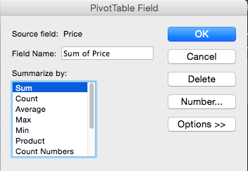
3. Click on the little “i” near the Price field and a new dialog will be shown like below. Select there the function “Sum”.

4.Format the PivotTable column to show nice $ formatted data.

You should get a report like this:

Now let’s extend this example and create a report showing Total and Average price by Geo/Channel.

We will continue from the previous report.

1. Open again the “PivotTable Builder” dialog by either clicking on the previous report or by navigating to the PivotTable tab option and clicking on the Builder icon.

2. Drag & Drop the “Channel” field to the “Row Labels”. Make sure it is the second row on that list.

3. Drag & Drop the “Price” field to the “Values”. Should now have two lines under “Values”.

4. Adjust the second “Price” line to use Average function. At this stage the Builder dialog should look like this:

5. Format the result report as needed.

You should have a report like this:

We are now masters of the simple PivotTable example.

Excel Icon Sets – Simple Example

They say that picture is worth a thousand words and that is even more accurate when dealing with numbers.

Sometimes in Excel you want to show Icons that provide quick meaningful indication for the value of the rows. A simple way to do that is by using Excel’s icon sets conditional formatting.

For a simple example, let’s assume that we have a table with product pipeline week-over-week and we want to provide visual indication if the pipeline is growing or declining using one of the following icons:

Let’s assume our pipeline table looks something like this:

And we want to add an icon beside the “Delta Prev Week” column with the icon.

To do that (on a Excel:Mac 2011) we will use conditional formatting:

1. In the menu select “Format” and then “Conditional Formatting…”. You should see the following popup:

2. Click on the Plus sign and select Style as “Icon Sets”.

3. Microsoft provides multiple predefined sets of icons so select the Icon Set that works best for your scenario. In this case we want use the arrows.

4. Setup the value ranges. In this case, everything above zero is green, zero is yellow and everything below zero is red. The result should be something like this:

5. Finally select the range for activating the conditional formatting by typing directly in the “Applies to” column. In this case I selected the entire column D:

6. The result is an icon assigned to column D with the needed icon:

There are also options to show only the icons and change the order of the icons.

See more information at Microsoft Office Talk here (It was written for Office 2007 for Windows but is still relevant).

Note that unfortunately at least in this release Microsoft does not provide an elegant way to load your own preferred icons. This is unfortunate and requires a weird workaround.

Excel VLookup – Simple Example

VLookup is an Excel search function. See the official definition at the Microsoft Office site. It is part of a family of search functions that includes Lookup, VLookup, HLookup and Match. Each one with a slightly different behavior.

The VLookup syntax seems abstract and complex so instead of explaining the syntax let’s focus on a use case:

Translation from key to its value. Such as in the case of translation from id to name.

For example, let’s assume in one place in the Excel worksheet we have a table of Customers that looks something like this:

The Customer table has pairs of Customer IDs and the associated Customer Names.

Now in a different place in the worksheet we have a Pipeline Table with Customer ID and Opportunity details. Something like this:

Note that in the Pipeline Table we have at column B the Customer ID. The big ask is to translate the Customer ID to Customer Name so that we can see who the customer in a more human readable fashion. See the empty column C above.

The VLookup for cell C2 will be as follows:
=VLOOKUP(B2,'Customer list'!A:B,2,TRUE)

Or in English:

• First parameter (B2): Take the value of cell B2
• Second parameter (‘Customer list’!A;B): Search for the first row containing this value in the “Customer list” table that has two columns. Column A and column B.
• Third parameter (2): When such row is found, use the second column (column B) of that row to place the value at C2.
• Fourth parameter (TRUE): The last parameter with value TRUE means that the search uses Exact match.

The final result is a new table with the customer name populated:

And that is the simple example of when and how to use VLookup.